A finite set of the states that each cell may be in
A partition of the cells into a uniform tessellation in which each tile of the partition has the same size and shape
A rule for shifting the partition after each time step
A transition rule, a function that takes as input an assignment of states for the cells in a single tile and produces as output another assignment of states for the same cells.
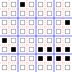
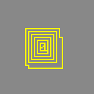
The simplest partitioning scheme is probably the Margolus neighborhood, named after Norman Margolus, who first studied block cellular automata using this neighborhood structure. In the Margolus neighborhood, the lattice is divided into 2-cell blocks (or 2 × 2 squares in two dimensions, or 2 × 2 × 2 cubes in three dimensions, etc.) which are shifted by one cell (along each dimension) on alternate timesteps.
The Margolus neighborhood for a two-dimensional block cellular automaton. The partition of the cells alternates between the set of 2 × 2 blocks indicated by the solid blue lines, and the set of blocks indicated by the dashed red lines.
The field
The field of the simulator is a rectangular lattice of cells, where each cell can be either dead or alive. The field is toroidal, that is: opposite edges of the field are “glued” together.
In the Margolus neighborhood, the lattice is divided into square blocks 2×2 cells. There are 2 partitioning schemes: in one scheme, top-left corner of each block has even coordinates, and in the another both coordinates are odd. These 2 schemes are alternated on each generation, first scheme is applied to the even generations, and second to the odd ones. Consequently, complete state of the field must also include the phase which is the oddity of the current generation.
Rules
Transition rule encoding
The transition rule is a function that calculated the next state of a block from the current state. For a cellular automaton to be reversible, such function should, indeed, be invertible.
Since in the Margolus neighborhood block consists of 4 cells and there are 2 possible cell states, 24 = 16 possible blocks exist:
0
1
2
...
15
...
Some of the possible block states.
A transition rule must assign a descendant state for each of the 16 original states. If the rule is invertible, this correspondence must be a one-to-one relation; in other words - it must be a permutation of 16 elements.
In the simulator, rules are represented as arrays of 16 integers from 0 to 15.
For example, (0,1,2,3,4,5,6,7,8,9,10,11,12,13,14,15,16) is the identity rule that does not changes any cells. The cellular automaton with this rule is rather boring though: in this rule, any pattern remains unchanged forever. This rule is, indeed, reversible.
More interesting example is the rule called “Billiard Ball Machine”. It is described by the permutation: (0,8,4,3,2,5,9,7,1,6,10,11,12,13,14,15). It is hard see from the numbers themselves, but this automaton exhibits behavior, resembling bouncing billiard balls and walls:
Behavior of the BBM cellular automaton resembles bouncing billiard balls.
Rule invariants
Contrary to the well-known Conway's Life cellular automaton, block automata with Margolus neighborhood has no (1,0) and (0,1) translation symmetry. This means that shift by 1 cell (or any other odd number of them) turns a pattern into completely different one. Only translation by a whole block (2 cells) in any direction leaves behavior of a pattern unchanged - it is guaranteed by construction.
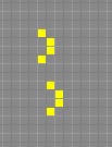
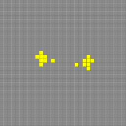
Top: P4 orthogonal spaceship. Bottom: P8 oscillator. The rule is “Critters&rdquo.
For example, in the “Critters” the top pattern is a spaceship, and the bottom is an oscillator.
Rules may have other invariants. The application performs analysis of a rule to determine them. The following invariants are detected:
Rotate by 90°
The rule has 4-fold rotational symmetry; transition function commutes with rotation by 90°.
For example, spaceship rotated by 90° will remain spaceship but change travel direction.
Rotate by 180°
The rule has 2-fold rotational symmetry; transition function commutes with rotation by 180°.
4-fold symmetry implies 2-fold too, but converse is not true. If a rule only have 2-fold symmetry, then spaceships in this rule
Horizontal / Vertical / Diagonal flip
The rule has mirror symmetry with axis, oriented horizontally, vertically or diagonally.
The “Critters” rule has mirror symmetry; mirrored pattern will evolve in the same way as original.
The “Rotations” rule (0,2,8,12,1,10,9,11,4,6,5,14,3,7,13,15) has no such symmetry. For example:
Left: P270 orthogonal c/135 spaceship. Right: P664 oscillator. (In the “Rotations” rule)
Negation
In the rules with negation symmetry, evolution of the pattern will be the same, if every alive cell is replaced with dead and back.
The “Rotations” rule is negation-invariant.
An inverted diagonal P9 spaceship: group of dead cells, traveling across the field of alive cells. “Rotations” rule.
Conservation law
Regarding the total number of alive cells in the field, 3 different kind of behavior can be observed:
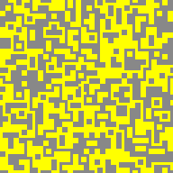
Number of alive cells varies.
“Tron” rule, (15,1,2,3,4,5,6,7,8,9,10,11,12,13,14,0) is an example of such behavior.
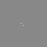
Evolution of the initial 3-cell pattern in the “Tron” rule on toroidal 64x64 field: initial pattern, after 12 steps, after 1200 steps
Usually, almost any initial pattern tends to grow chaotically in such automata. Numbers of dead and alive cells tending to become nearly equal. Often, resulting pattern is visually indistinguishable from the random noise, though the “Tron” rule is a counter-example.
Number of alive cells is constant.
“Billiard Ball Machine” rule is an example.
“Flashing” rules, where numbers of alive and dead cells are interchanging on each generation.
After 2 generations, number of alive cells returns to the original value, so it can be considered as a special case of the previous type.
The “Critters” rule is an example.
Dual transform
Time-inverted block cellular automaton is also block cellular automaton of the same kind.
Its rule is inverse permutation of the original rule.
However, there is one more difference: in time-inverted cellular automata, order of phases of the lattice is also inverted. This can be obtained by translating whole field by 1 cell along both axes. In the simulator program, this is called phase shift; buffer content can be phase-shifted with button (Phase).
In a general case, the inverse rule is completely different from the direct. But for some rules, a simple geometrical relation between direct and inverse rules is present. For example, in the “Rotations” rule (0,2,8,12,1,10,9,11,4,6,5,14,3,7,13,15) inverse rule is a mirror image of the direct. In other words, to inverse-transform a pattern, one could first mirror it, then transform it directly, and finally mirror it again. It can be written down as:
F-1(x) = H-1(F(H(x))) = (H-1∘F∘H)(x),
or:
F-1 = H-1∘F∘H,
where F is a cellular automaton transition function; H is some geometrical transform, horizontal flip in this case; x is a field state and ∘ designates composition of functions. I call the transform H, satisfying the above relation, a dual transform for the rule F.
If dual transform exists for a rule, then for every pattern it is possible to construct a dual pattern that evolved back in time.
It can be constructed in following 2 steps:
apply dual transform to the pattern,
offset transformed pattern by the vector (1,1) (“phase shift”).
Example:
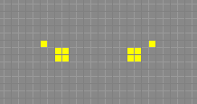
A P9, c/9 spaceship (left) and its dual (right), in the “Rotations” rule. Dual transform is mirror flip.
Note the direction of the dual (left) spaceship. It moves in a direction, opposite to the flipped direction of the original spaceship, because it evolves back in time.
For some rules, dual transform is identity. I call such rules self-dual, example is the “Critters” rule. In such rules, it is enough to phase-shift a pattern to construct its dual.
Rule vacuum period
Number of generations, after which empty field (vacuum) returns to its original state. For the population-preserving rules, vacuum period is 1; for the “flashing” rules it is 2. Some irregular rules can have bigger vacuum periods. For example, asymmetric rule (1,2,3,4,5,6,7,8,9,10,11,12,13,14,15,0) has vacuum period of 7.
Predefined Rules
The simulator contains a set of predefined rules, taken from the MCells page.
Here are they:
Name
Rule
Description
BBM
0,8,4,3,2,5,9,7,1,6,10,11,12,13,14,15
Famous Billiard Ball Machine - from Cellular Automata Machines. A rule by Edward Fredkin.
Bounce Gas
0,8,4,3,2,5,9,14,1,6,10,13,12,11,7,15
An uniform “gas”. A rule by Tim Tyler.
Bounce Gas II
0,8,4,12,2,10,9,7,1,6,5,11,3,13,14,15
Another uniform “gas”. A rule by Tim Tyler.
Critters
15,14,13,3,11,5,6,1,7,9,10,2,12,4,8,0
This rule supports “gliders” - as described in Cellular Automata Machines. A rule by Margolus/Toffoli.
HPP Gas
0,8,4,12,2,10,9,14,1,6,5,13,3,11,7,15
HPP (Hardy/Pazzis/Pomeau) lattice gas - as described in Cellular Automata Machines. A rule by Hardy, Pazzis, and Pomeau.
Rotations
0,2,8,12,1,10,9,11,4,6,5,14,3,7,13,15
Limited diffusion. A rule by Tim Tyler.
Rotations II
0,2,8,12,1,10,9,13,4,6,5,7,3,14,11,15
Limited diffusion. A rule by Tim Tyler.
Rotations III
0,4,1,10,8,3,9,11,2,6,12,14,5,7,13,15
Slow, random-looking diffusion. A rule by Tim Tyler.
Rotations IV
0,4,1,12,8,10,6,14,2,9,5,13,3,11,7,15
Slow, random-looking diffusion. A rule by Tim Tyler.
Sand
0,4,8,12,4,12,12,13,8,12,12,14,12,13,14,15
Sand simulation. Non-revertible. A rule by Mirek Wojtowicz.
String Thing
0,1,2,12,4,10,9,7,8,6,5,11,3,13,14,15
String shaped patterns. A rule by Tim Tyler.
String Thing II
0,1,2,12,4,10,6,7,8,9,5,11,3,13,14,15
More string shaped patterns. A rule by Tim Tyler.
Swap On Diag
0,8,4,12,2,10,6,14,1,9,5,13,3,11,7,15
A gas with no particle interactions - as described in Cellular Automata Machines. A rule by Margolus/Toffoli.
Tron
0,15,1,2,3,4,5,6,7,8,9,10,11,12,13,14,0
A “trip-a-tron” - from the pages of Cellular Automata Machines. A rule by Margolus/Toffoli.
RLE encoding
For textual representation of the patterns, the simplified RLE format is used. RLE string consists of decimal numbers and characters “b”, “o” and “$”, designating dead cell, alive cell and new line correspondingly. Decimal numbers designate repeat count of the next character.
See details here. Only “b” (dead cell), “o” (alive cell) and “$” (newline) characters and digits are supported; space characters are ignored. Example:
Conway GOL glider. RLE encoding is 2o$obo$o.
Comments, offset and other features of RLE are not supported.
Features
Pattern analyzer
Some rules (such as Rotations, Rotations II, III, IV) support spaceships and oscillators with extremely large periods.
For example, The following spaceship in the “Rotations II” rule (0,2,8,12,1,10,9,13,4,6,5,7,3,14,11,15) has period 10896 generations.
A spaceship with period 10896. Rule is “Rotations II”
Manual classification of such patterns is nearly impossible. To simplify this task, the simulator has the pattern analyser feature, enabled by the (AS) button. To use it, select some area on the field and then press the button. Application will try to detect the following information:
Type of the pattern: oscillator, diagonal, orthogonal or slant spaceship.
Period (for the spaceships and oscillators).
Offset (for the spaceships): how far the spaceship travels per one period.
Canonical form of the pattern: the most “compact” of all evolution steps of the pattern. Sometimes it is not unique.
Analyzer only tries to evaluate a pattern for a limited number of generations. If this number is exceeded before the cycle is found, pattern type and period will be shown as “unknown”. By default, limit is 2048 steps, this value can be changed on the “Settings” panel.
Spaceship Catcher
Enabled by the button: (Catcher).
Spaceship catcher is a tool that automatically :
finds all patterns touching the borders of the field,
removes them from the field,
analyses and adds canonical form to the current library.
When enabled, spaceship catcher reseeds the field periodically: the field is cleared and currently selected area is filled randomly. By default, reseed period is 30'000 generations, it can be changed in the “Settings” panel.
Spaceship catcher can be used to quickly find naturally occurring gliders for the given rule.
GIF Recorder
The application can record GIF animations. To start record, press the R. This will start the recorder. Then let the field evolve for several generations, using play buttons. Each new frame will be added to the GIF image. You will see, how the size of the file in Kb grows. To stop record and get the produced image, press the S button. Image can be saved using right-click.
Patterns Library
The simulator support simple management of pattern libraries: catalogs of patterns. Libraries are stored in the Local Storage of the browser, and will remain there even after restart of the browser. To move library between browsers, or to analyze library data with another application, JSON import/export feature is available.